NFL WR Injury Analysis

Exploring whether height and weight are associated with season-ending injuries among notable NFL wide receivers (2016–2026), motivated by the Chargers drafting Brennan Thompson — an extreme outlier by size.

Background

The Los Angeles Chargers made headlines by selecting Brennan Thompson — a wide receiver listed at just 5’9” and 164 lbs — in the 2026 NFL Draft. At those measurements, Thompson is a genuine outlier among NFL wideouts: lighter than any established receiver in recent memory and among the shortest in the league.

This raises a natural question: do smaller, lighter receivers get hurt more often? To explore it, I assembled a dataset of 170 notable NFL wide receivers from 2016–2026 and looked at whether physical size correlates with season-ending injury rates. No modeling — just the data and clean visualizations.

Data

library(tidyverse)

df <- read_csv("../assets/NFL_WR_injury_data.csv") %>%
  rename(Injured_raw = `Season-Ending Injury`) %>%
  mutate(
    Height_in = {
      m <- str_match(Height, "(\\d+)'(\\d+)")
      as.numeric(m[, 2]) * 12 + as.numeric(m[, 3])
    },
    Weight_lbs = as.numeric(str_extract(Weight, "\\d+")),
    Injured = if_else(Injured_raw, "Season-Ending Injury", "Not Injured"),
    Injured = factor(Injured, levels = c("Not Injured", "Season-Ending Injury"))
  )

brennan <- df %>% filter(Player == "Brennan Thompson")

cat(sprintf(
  "Dataset: %d receivers | %d with season-ending injuries (%.0f%%)\n",
  nrow(df), sum(df$Injured_raw), mean(df$Injured_raw) * 100
))

Dataset: 166 receivers | 74 with season-ending injuries (45%)

The dataset covers 166 notable NFL wide receivers with documented injury histories from 2016–2026. Each player is coded as having suffered a season-ending injury (TRUE) or not (FALSE) during that window. Height and weight are parsed from their string formats into numeric values for analysis.

Analysis

Height vs. Weight — Where Does Thompson Fit?

pal <- c("Not Injured" = "#013369", "Season-Ending Injury" = "#D50A0A")

fmt_height <- function(x) paste0(x %/% 12, "'", x %% 12, '"')

ggplot(
  df %>% filter(Player != "Brennan Thompson"),
  aes(x = Weight_lbs, y = Height_in, color = Injured)
) +
  geom_point(size = 3, alpha = 0.72) +
  geom_point(
    data = brennan,
    aes(x = Weight_lbs, y = Height_in),
    color = "#FFB612", size = 6, shape = 18, inherit.aes = FALSE
  ) +
  geom_label(
    data = brennan,
    aes(x = Weight_lbs, y = Height_in, label = "Brennan Thompson\n5'9\", 164 lbs"),
    color = "black", fill = "#FFB612", fontface = "bold",
    size = 3.4, nudge_y = 1.7, nudge_x = 6,
    inherit.aes = FALSE
  ) +
  scale_color_manual(values = pal) +
  scale_y_continuous(breaks = seq(66, 78, 2), labels = fmt_height) +
  labs(
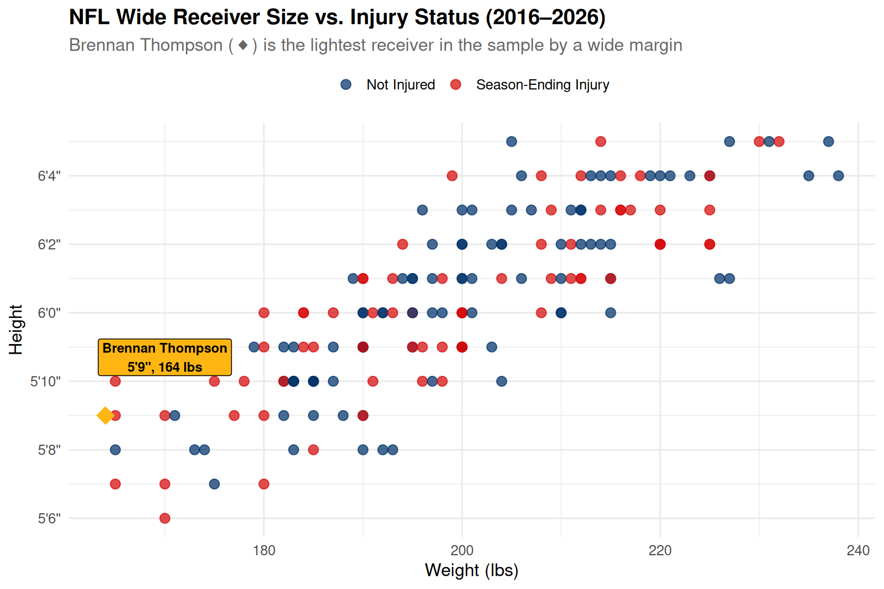
    title = "NFL Wide Receiver Size vs. Injury Status (2016–2026)",
    subtitle = "Brennan Thompson (◆) is the lightest receiver in the sample by a wide margin",
    x = "Weight (lbs)", y = "Height",
    color = NULL
  ) +
  theme_minimal(base_size = 13) +
  theme(
    legend.position = "top",
    plot.title = element_text(face = "bold"),
    plot.subtitle = element_text(color = "gray40")
  )

Thompson sits well below and to the left of the entire sample. There is no comparable player in this dataset — at 164 lbs, he is more than 15 lbs lighter than the next lightest receiver. The scatter also shows that injured and non-injured players are broadly intermixed across the size spectrum, with no obvious clustering pattern.

Distribution by Injury Status

pal_fill <- c("Not Injured" = "#013369", "Season-Ending Injury" = "#D50A0A")

box_theme <- theme_minimal(base_size = 13) +
  theme(plot.title = element_text(face = "bold", size = 12))

print(
  ggplot(df, aes(x = Injured, y = Height_in, fill = Injured)) +
    geom_boxplot(alpha = 0.75, outlier.shape = 21, outlier.fill = "white") +
    scale_fill_manual(values = pal_fill, guide = "none") +
    scale_y_continuous(breaks = seq(66, 78, 2), labels = fmt_height) +
    labs(title = "Height by Injury Status", x = NULL, y = "Height") +
    box_theme
)

print(
  ggplot(df, aes(x = Injured, y = Weight_lbs, fill = Injured)) +
    geom_boxplot(alpha = 0.75, outlier.shape = 21, outlier.fill = "white") +
    scale_fill_manual(values = pal_fill, guide = "none") +
    labs(title = "Weight by Injury Status", x = NULL, y = "Weight (lbs)") +
    box_theme
)

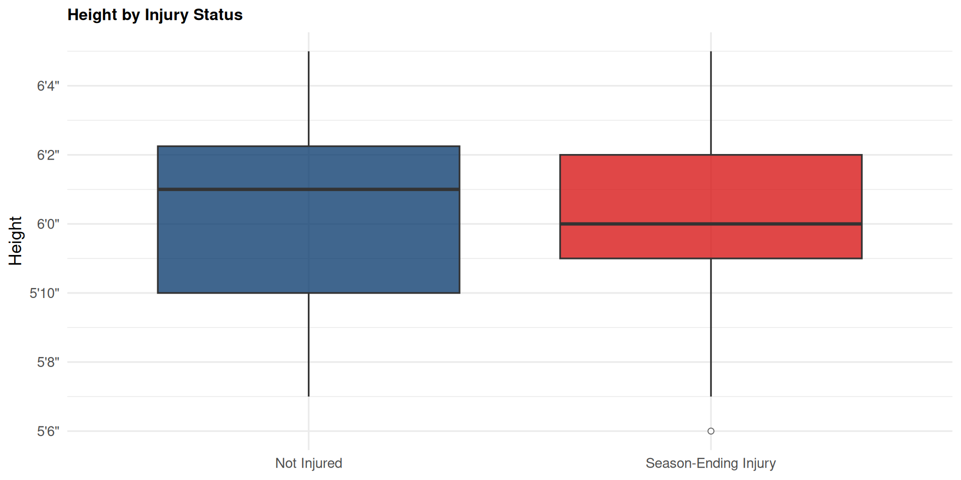
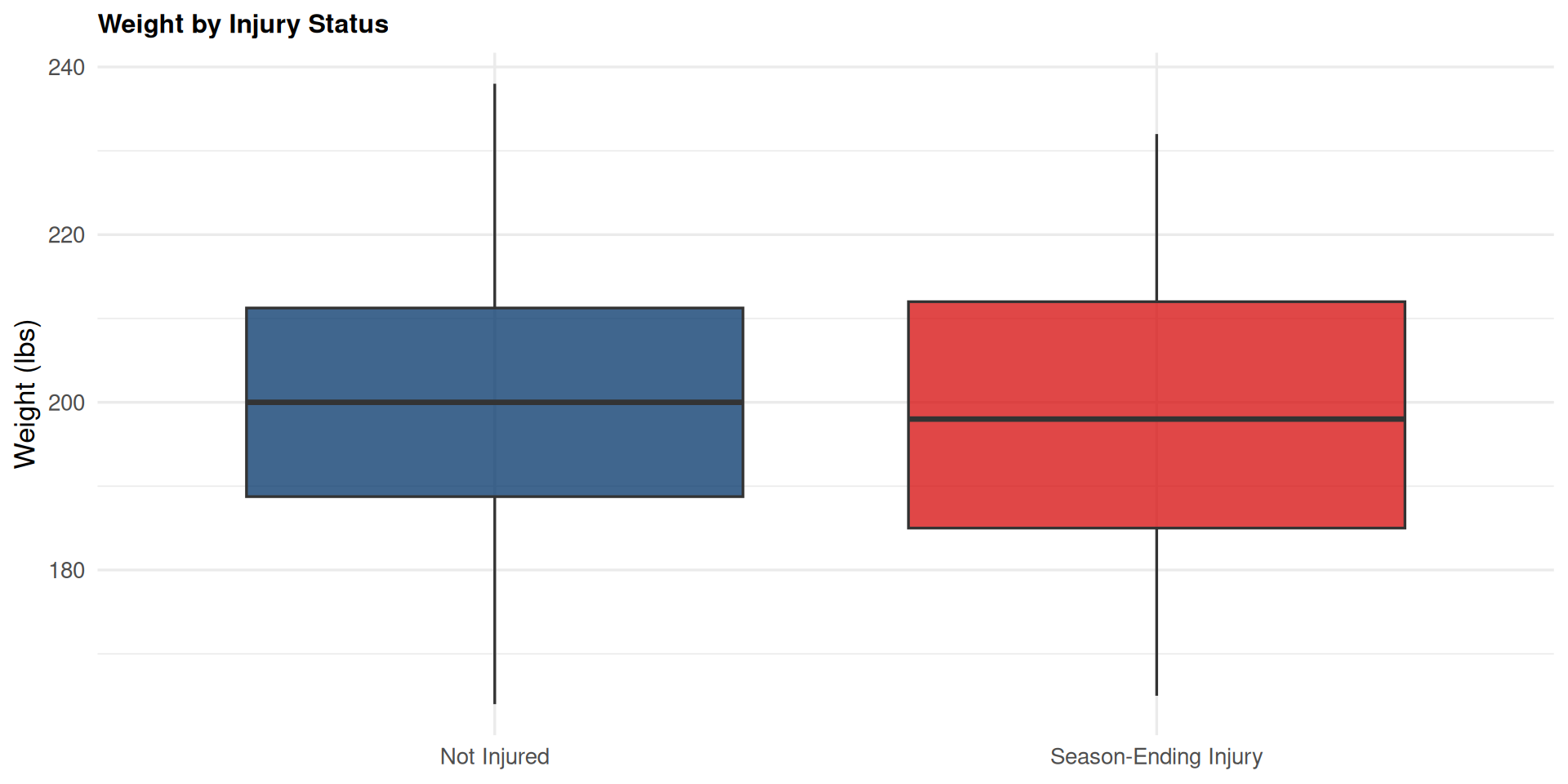
The medians are close between groups for both height and weight. The injured group shows slightly wider spread — particularly at the upper end of the weight range — but there is no dramatic size difference between the two populations.

Injury Rate by Size Group

med_h <- median(df$Height_in)
med_w <- median(df$Weight_lbs)

df_g <- df %>%
  mutate(
    Height_group = if_else(
      Height_in >= med_h,
      paste0("Tall (≥ ", fmt_height(med_h), ")"),
      paste0("Short (< ", fmt_height(med_h), ")")
    ),
    Weight_group = if_else(
      Weight_lbs >= med_w,
      paste0("Heavy (≥ ", med_w, " lbs)"),
      paste0("Light (< ", med_w, " lbs)")
    )
  )

rate_h <- df_g %>%
  group_by(Height_group) %>%
  summarize(rate = mean(Injured_raw) * 100, n = n(), .groups = "drop") %>%
  mutate(Height_group = fct_reorder(Height_group, -rate))

rate_w <- df_g %>%
  group_by(Weight_group) %>%
  summarize(rate = mean(Injured_raw) * 100, n = n(), .groups = "drop") %>%
  mutate(Weight_group = fct_reorder(Weight_group, -rate))

bar_theme <- theme_minimal(base_size = 13) +
  theme(
    plot.title = element_text(face = "bold", size = 12),
    panel.grid.major.x = element_blank()
  )

print(
  ggplot(rate_h, aes(x = Height_group, y = rate, fill = rate)) +
    geom_col(alpha = 0.88, width = 0.55) +
    geom_text(
      aes(label = sprintf("%.0f%%\n(n=%d)", rate, n)),
      vjust = -0.35, fontface = "bold", size = 4
    ) +
    scale_fill_gradient(low = "#013369", high = "#D50A0A", guide = "none") +
    ylim(0, 72) +
    labs(title = "Injury Rate by Height Group", x = NULL, y = "% with Season-Ending Injury") +
    bar_theme
)

print(
  ggplot(rate_w, aes(x = Weight_group, y = rate, fill = rate)) +
    geom_col(alpha = 0.88, width = 0.55) +
    geom_text(
      aes(label = sprintf("%.0f%%\n(n=%d)", rate, n)),
      vjust = -0.35, fontface = "bold", size = 4
    ) +
    scale_fill_gradient(low = "#013369", high = "#D50A0A", guide = "none") +
    ylim(0, 72) +
    labs(title = "Injury Rate by Weight Group", x = NULL, y = "% with Season-Ending Injury") +
    bar_theme
)

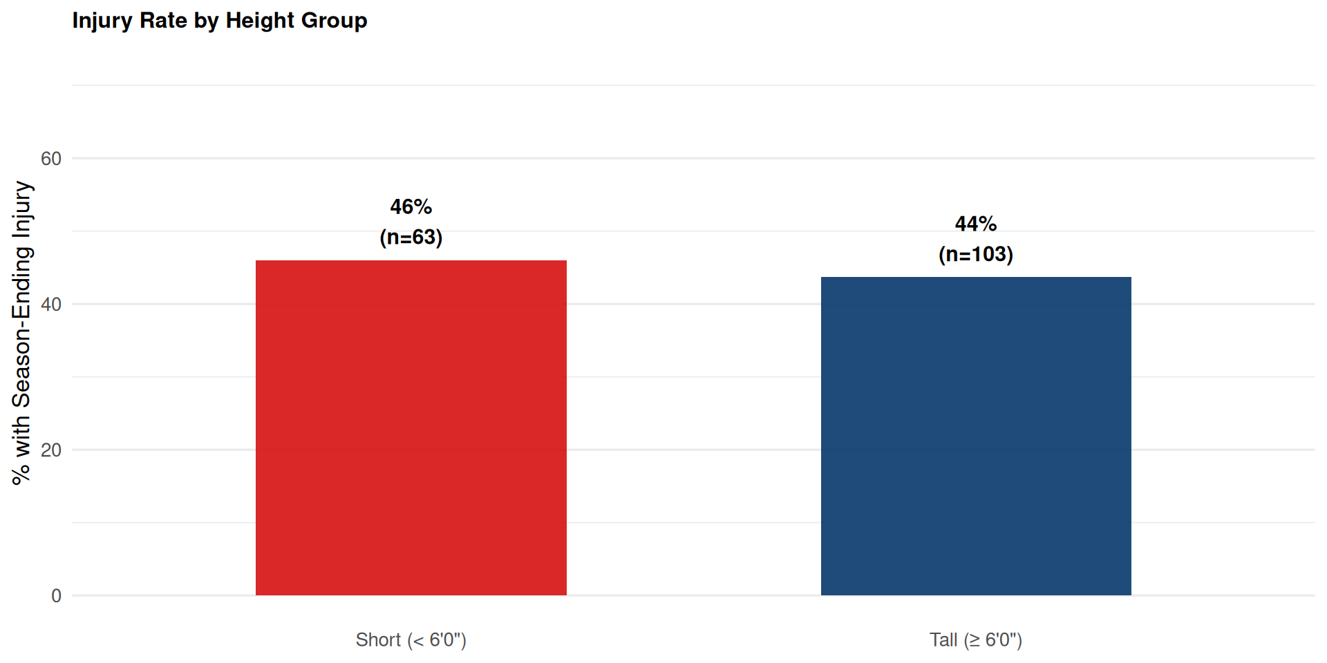
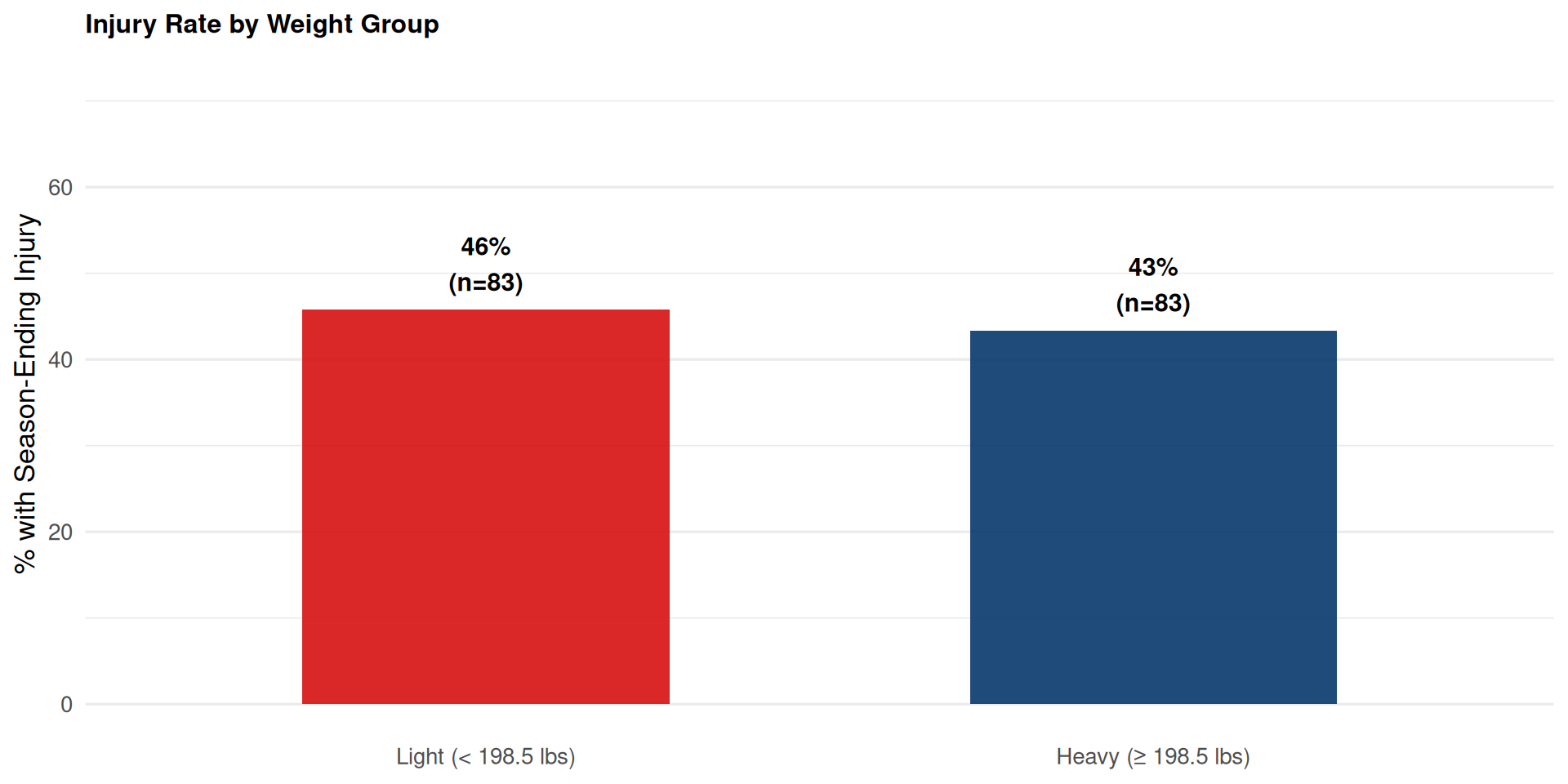
When splitting at the median, a counterintuitive pattern emerges: taller and heavier receivers show higher injury rates in this sample. This cuts against the intuition that smaller receivers might be more fragile. That said, the groups are roughly equal in size and the differences are modest — strong conclusions require more data and controls.

Weight Distribution: Injured vs. Not Injured

ggplot(df, aes(x = Weight_lbs, fill = Injured, color = Injured)) +
  geom_density(alpha = 0.35, linewidth = 1) +
  geom_vline(
    xintercept = brennan$Weight_lbs,
    linetype = "dashed", color = "#B8860B", linewidth = 1
  ) +
  annotate(
    "text", x = brennan$Weight_lbs + 3, y = 0.025,
    label = "Thompson\n164 lbs", hjust = 0,
    color = "#8B6914", fontface = "bold", size = 3.6
  ) +
  scale_fill_manual(values = pal_fill) +
  scale_color_manual(values = pal_fill) +
  labs(
    title = "Weight Distribution: Injured vs. Not Injured Receivers",
    subtitle = "Brennan Thompson falls well below the bulk of both distributions",
    x = "Weight (lbs)", y = "Density",
    fill = NULL, color = NULL
  ) +
  theme_minimal(base_size = 13) +
  theme(
    legend.position = "top",
    plot.title = element_text(face = "bold"),
    plot.subtitle = element_text(color = "gray40")
  )

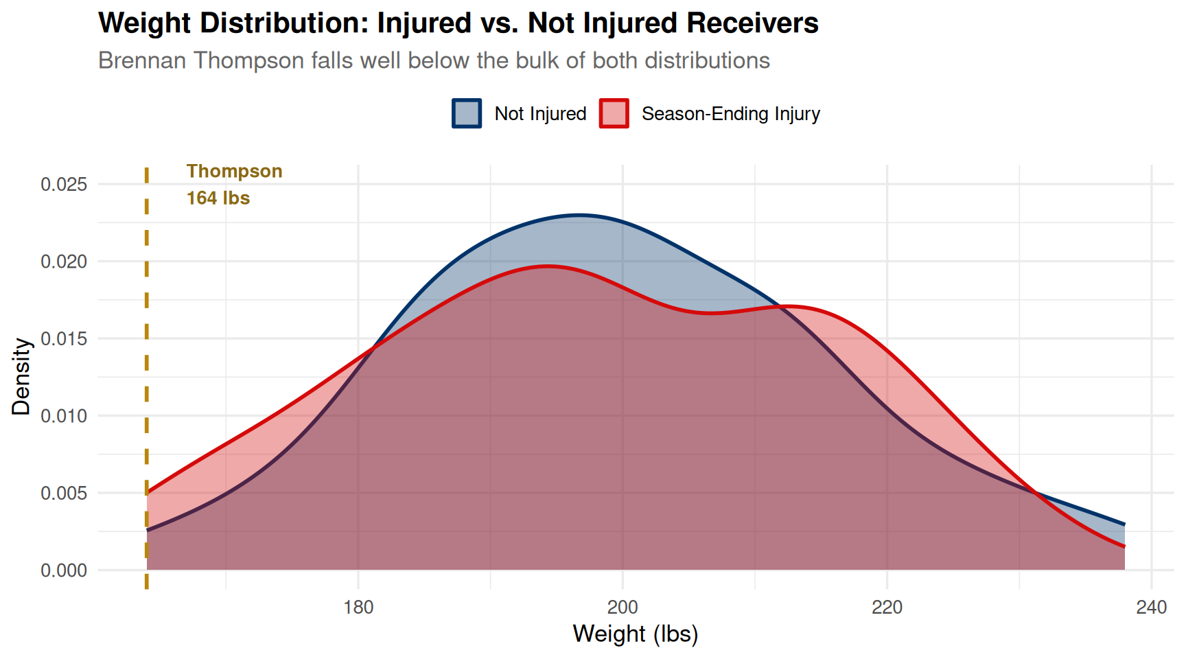
Both distributions peak around 195–215 lbs and overlap substantially — weight alone is not cleanly separating injured from non-injured receivers. Thompson’s 164 lbs sits far to the left of both curves, in territory with no historical precedent in this sample.

Takeaways

• At 5’9”, 164 lbs, Brennan Thompson is a genuine outlier — no comparable receiver appears in this sample of 170 notable NFL wideouts over the past decade.
• Size alone does not predict season-ending injuries in this data: the distributions between injured and non-injured groups overlap heavily.
• If anything, larger receivers show slightly higher injury rates when split at the median, which runs counter to the “fragile small receiver” narrative.
• The more meaningful concern for Thompson may not be injury frequency but durability at the point of contact — a question this dataset can’t answer without play-type and contact data.

This is an exploratory, descriptive analysis. With ~170 players and no controls for position role, snap count, age, or playing style, these patterns are observational — not causal.